An intuitive way to understand information
Published:
This post proposes a way to intuitively grasp the idea of information and presents a package to perform the deduction behind the idea. Some experiment results are also shown in this post.
Idea in one sentence
Information is simply a one to many relationship. For example, when we say we see a bird, it could be a sparrow, a crow, or an eagle, etc. This set of numerous species is equivalent to the concept of bird. When we say an old lady is cooking in a cold morning, we think of numerous scenes that fit this sentence. In a neural network, if some hidden layer outputs a certain vector, the set of input vectors that all propagate to this vector is equivalent to this vector.
Dig deeper into the neural network case
Let’s say I have a pretrained CNN classification network. And I fixed the output to [0, 1, 0, 0], which is the labels of bird. Applying the above concept, the concept of [0, 1, 0, 0] is equivalent to the set of input pictures that all propagate to this value. Let’s call this input set the solution set. In pratice these neural networks always output values close to [0, 1, 0, 0], but this doesn’t affect our analysis, since we can add a final approximation layer.
How do we get the solution set?
- In a neural network, a hidden layer is just a group of mathematical expressions. When we want to get all inputs that eventually forward propagate to certain hidden layer value, we are actually trying to solve a system of mathematical expressions.
- The algorithm of solving the equations is as follows:
**Natural Language Format**
1. The set that contains only our desired output is the initial output set
2. For a certain layer, find all solutions that forward propagate to the valid output set. Take the intersection of the solutions and the range of the previous layer as the valid output set for the previous layer.
3. Loop the above procedure through the neural network backwards
4. The solution set of the first layer is the solution set of the neural network with respect to our desired output

**Pseudo Code Format**
# this function finds all solutions of a certain layer given a certain output
def find_all_solutions_of_certain_layer(layer, output):
    ### implementation
    return solution_set

# this function finds the range of a certain layer while all its inputs can move freely
def find_the_range_of_certain_layer(layer):
    ### implementation
    return range

layer_list = [Linear(64, 32), ReLU, Linear(32, 10), Softmax]   # only an example
layer.reverse()   # reverse the neural network, since our solving process is backward
output_set = ([0.02, 0.82, 0.02, 0.02, 0.02, 0.02, 0.02, 0.02, 0.02, 0.02])   # only an example, the initial set only contains one element, which is our ultimate required output

# loop through the neural network backwards
for layer in layers:
    layer_range = find_the_range_of_certain_layer(layer)
    valid_output_set = intersection(output_set, layer_range)
    solutions = []
    for output in valid_output_set:   # for every output in the valid set, find its solution set and combine them together
        solutions.append(find_all_solutions_of_certain_layer(layer, output))
    output_set = union(solutions)

input_set = output_set  # solved!
- The full version of the above algorithm is theoretically right but impossible to implement in reality. We can modify the algorithm a little bit so that it becomes implementable:
- When finding solutions of a certain layer with respect to a particular output, we don’t find all of them. We only sample some solutions.
- The details of the implementation are in the Appendix.
- The repo link: https://github.com/scottyaohk/Back-solve-neural-network
What does the solution set look like?
- Let’s first look at an experiment of the above algorithm:
- Steps
- Take a 2-layer fully connected network trained on MNIST dataset as an example.
- The network structure is as follows: [Linear(784, 256), LeakyReLu(0.01), Linear(256, 10), Softmax]
- After training, the network reaches an accuracy of 94.31% on test dataset.
- Randomly pick a picture from test dataset. Forward propagate the picture through the network. Record the final output.
- Back-solve the network with respect to the output mentioned above.
- Take a 2-layer fully connected network trained on MNIST dataset as an example.
- Results
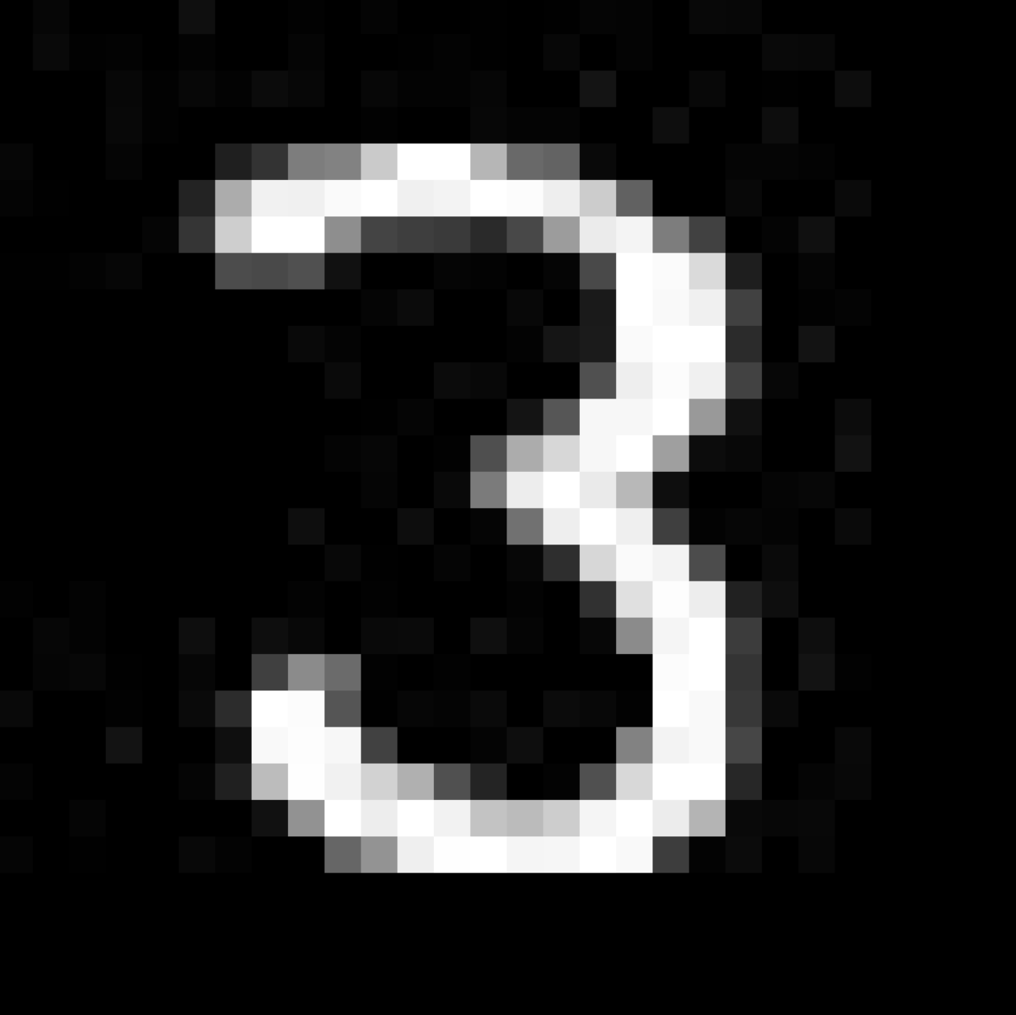
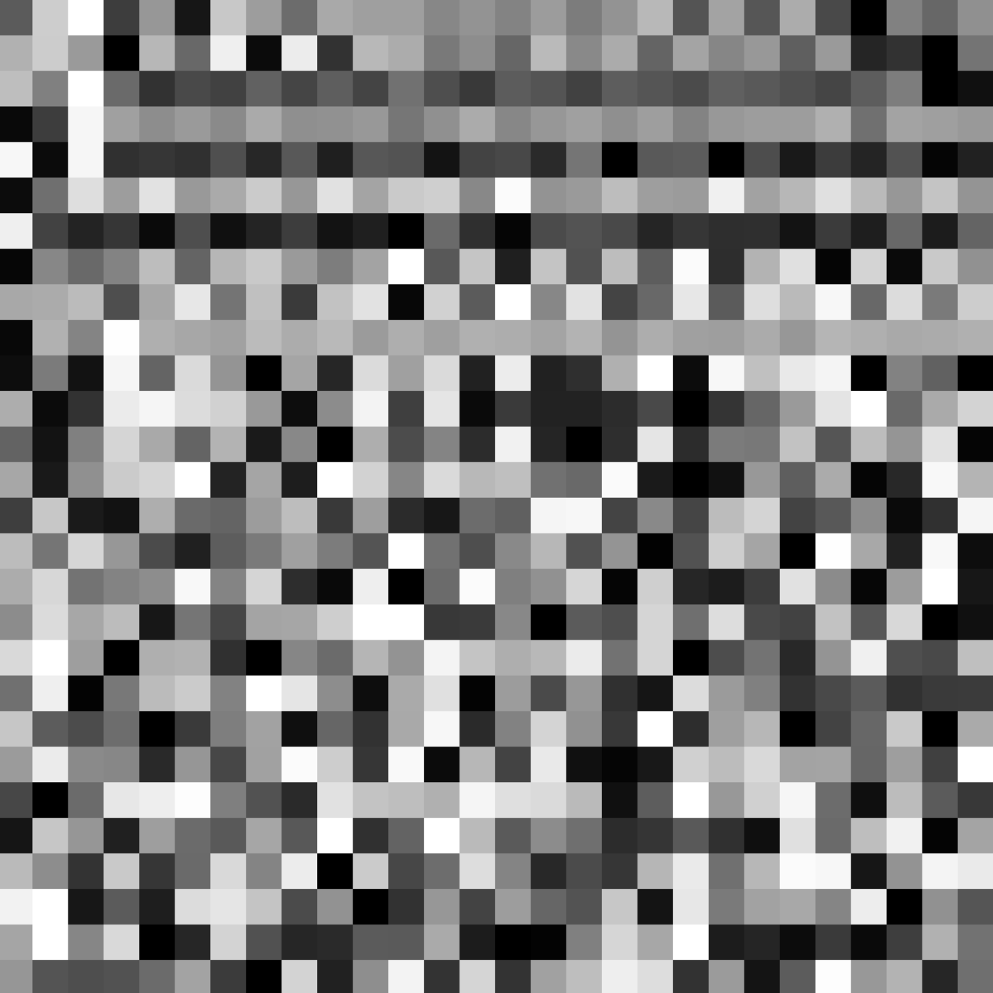
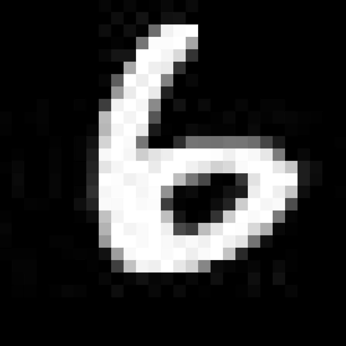
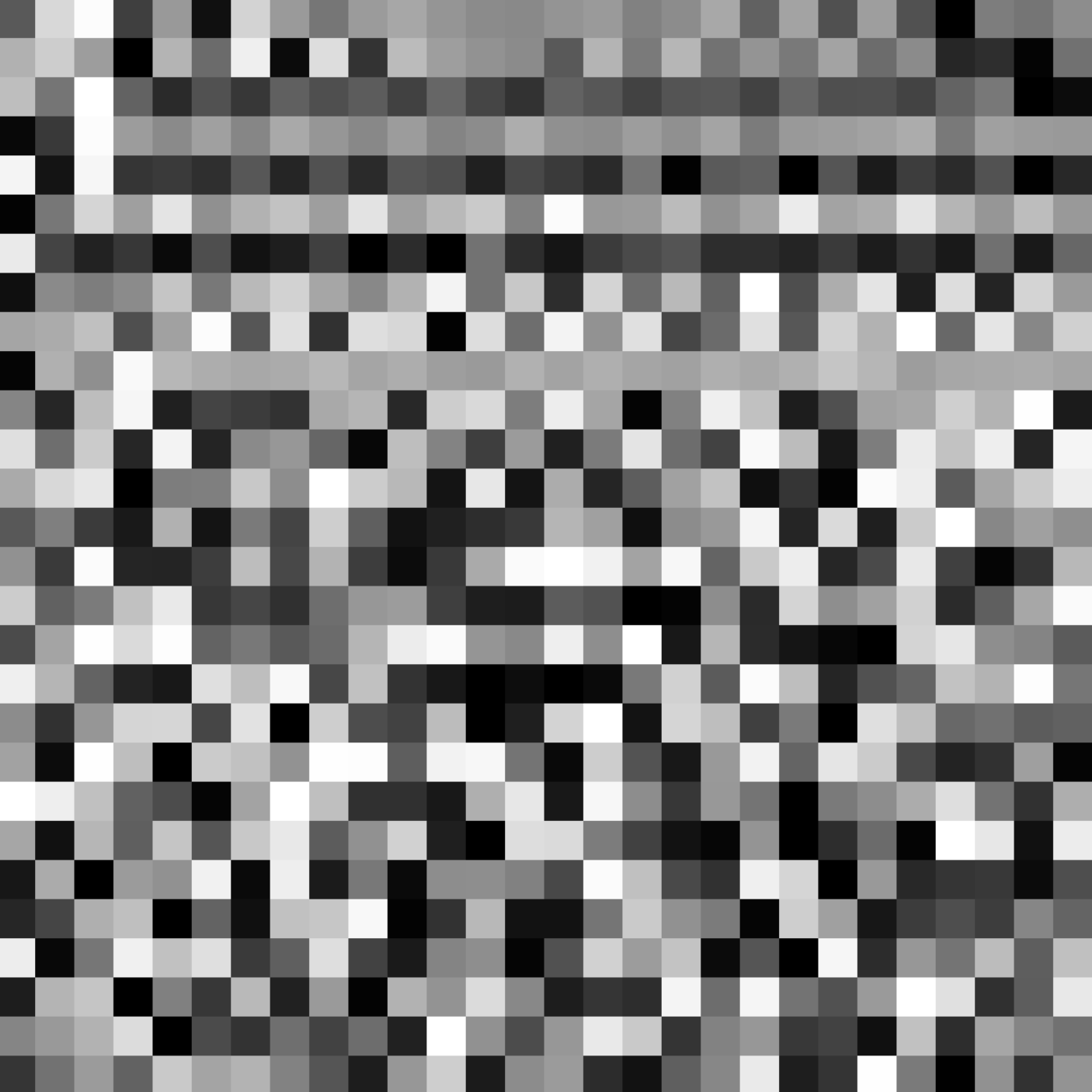
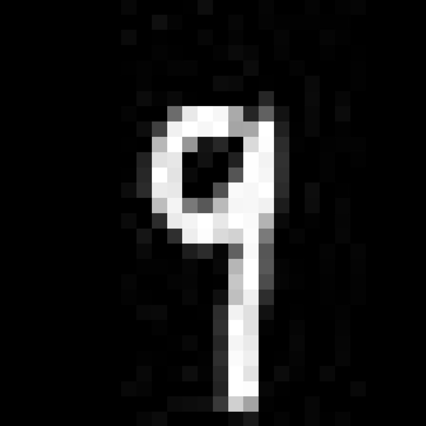
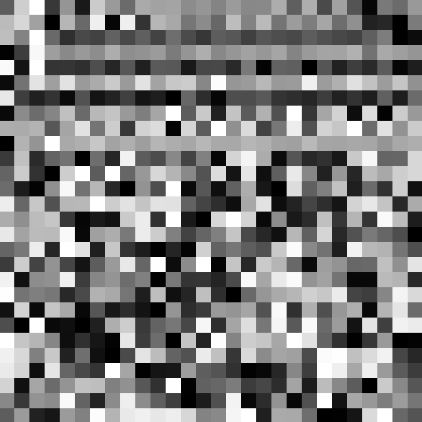
- The left one is the randomly picked picture from test dataset. The right one is the solution input with respect to the output of the left one.
- Findings
- Although the left and the right pictures share the same output, the right one looks nothing like the left one.
Now let’s go back to the question of what the solution set looks like.
- Imagine the shape of the solution input set
- It is easier to first imagine the shape of the solutions of a linear layer.
- Below is the uniform formula of linear equations: \(x = x_s + \sum_i\epsilon_i * x_i\)
- \(x_s\) represents the special solution, \(x_i\) represents all null solutions, \(\epsilon_i\) represents arbitrary number within \(R\). The number of \(x_i\) equals the number of free variables, which is smaller than the dimension of \(x\).
- Suppose the number of free variables is \(n\) and the dimension of \(x\) is \(m\) (\(m > n\)). Then the solution set of the linear layer is just a n-dimensional linear-shaped space in \(R^m\) space.
- In \(R^2\), it is a line, a dot or an empty set. In \(R^3\), it is a plane, a line, a dot or an empty set. We are able to get a very intuitive idea of what it looks like even in high dimensional space. It is linear and it stretches across the whole space.
- Usually, we would have multiple outputs to back-solve in the middle of the neural network. In this case, the solution set of all valid outputs is just the union of different solution set of every valid output. After the union, many properties of a single solution set still remains, like some linear structure and the boundless stretching.
- Now let’s examine what role the nonlinear layer is playing.
- Take ReLU as an example.
- When back-solving the ReLU layer, for every element, as long as it is positive, the corresponding solution element is definite. If it is zero, the corresponding element can be any non-positive number. If it is negative, there are no corresponding solution. Imagine in a \(R^3\) space, the solution is a 2D plane. The plane crosses “zero-plane” at some line. Everything on this plane after this line will be truncated since it is unreachable by ReLU function. Every point on the line will be extended vertically downward. So the solution set will be a bent plane. Nonlinearity is added and this nonlinearity will be remembered when back-solving through further layers.
- Take ReLU as an example.
- Up to this point, I believe we could get a very intuitive idea about why the solution picture looks nothing like the original one.
- The solution set is not a perfect copy of the distribution that we human take for granted. Instead, it just contains the pictures of a certain number within a predetermined distribution, usually, the pictures that are naturally generated. The true solution set is extremely complex and is the product of all those linear layers and nonlinear layers. It includes many other irrelevant candidates unavoidably.
- The reason why neural network still works very well is that the inputs we usually feed in a network are already in the set of all naturally generated pictures.
- It is easier to first imagine the shape of the solutions of a linear layer.
After thinking through the above things, I find many odd behaviors of neural networks intuitive.
- For example, we could fool the neural network to recognize an elephant as a koala by adding a tiny noise. And the two pictures look almost the same.
- I think this is due to the extremely complex solution structure. What the network actually recognizes as a koala is a set containing both the normal koala pictures generated naturally and other solutions that radiate through the whole space. There are many solution candidates of koala just near an ordinary elephant picture. However, they are all beyond the normal scope of naturally generated pictures, which means they won’t interfere with the use of neural network.


elephant, according to VGG16 pretrained on Imagenet
koala, according to VGG16 pretrained on Imagenet

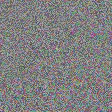
the difference between the above two pictures
the difference after maginified ten times
Appendix
Back-solver Doc
- To facilitate finding the one-to-many relationship mentioned above, I wrote a tiny package for this specific use. For every layer, the package basically computes the solutions with respect to the required layer output. And this process is repeated from the last layer to the first layer. The intersection of all solutions of a certain layer and the range of the previous layer is the valid output of the previous layer. The solution set of the first layer is the solution of the whole neural network with respect to the initially dictated last layer output.
- The core of this package is a linear equation system solver using Gaussian elimination method. I implemented this solver using purely numpy basic methods. The linear solver is responsible for the “back-solving” process of all Linear layers and other layers that involves linear equations, like Softmax.
- Precision plays a very important role in solving linear equations, since the computer performs finite digit operations at the very bottom. According to my experiment, when the matrix gets bigger and complex, low precision will result in answers that have non-negligible error. The solution is to use high enough precision. I used numpy.float64, which worked well in my experiment context.
- Another thing to mention is that this solver couldn’t solve every linear equations. For those systems that will encounter absolute zero during elimination, the finite nature of computer will sometimes result in a non-zero number where it should be a zero instead. This makes a huge difference. Because it can’t be mitigated by increasing the precision. Luckily, the probability that we encounter this type of situation is zero. So we can just ignore this scenario and apply Gaussian elimination on the computer anyway.
- In the engine.py, I wrote the base class that is responsible for sample solutions from the solution set. For every type of neural network layer, we could implement a subclass that performs the “back-solving” and “sampling” steps. I only implement the subclass for linear layer, softmax, relu and leaky relu.
- The package is incomplete in the following aspects:
- The sampling method needs to be further studied.
- We need a way to constrain the sampled solutions to be in a certain range, since layers like relu only output values in a give range.
- More subclasses to be implemented
- More robust linear equation system solver needed
- …
- Here is the repo link to the package:
- https://github.com/scottyaohk/Back-solve-neural-network
